Calculate Bessel-Ie Function
Online calculator for the exponentially scaled modified Bessel function Ieᵥ(z) - Numerically stable for large arguments
Bessel-Ie Function Calculator
Exponentially Scaled Bessel Function
The Ieᵥ(z) or exponentially scaled modified Bessel function provides numerical stability for large arguments.
Bessel-Ie Function Curve
Mouse pointer on the graph shows the values.
The exponentially scaled form is numerically more stable for large z.
|
|
Why exponential scaling?
The exponentially scaled modified Bessel function solves numerical problems:
- Numerical stability: Prevents overflow for large z
- Exponential factor: Ieᵥ(z) = e^(-z) Iᵥ(z)
- Precision: Maintains accuracy for all z ranges
- Implementation: Standard in numerical libraries
- Range extension: Computation for very large arguments
- Robustness: Avoids machine precision problems
Numerical advantages over standard Bessel-I
The exponentially scaled version offers crucial numerical advantages:
Problem with standard Iᵥ(z)
- Exponential growth ~ e^z
- Overflow at z > ~700
- Loss of precision
Solution through Ieᵥ(z)
- Scaled range without overflow
- Stable computation for all z
- Preserved relative accuracy
Formulas for the Bessel-Ie Function
Definition
Exponentially scaled modified Bessel function
Relationship to Iᵥ
Inversion of scaling
Series Expansion
Scaled power series
Asymptotic Form
For large z (without exponential growth)
Recurrence Formula
Same recurrence as unscaled version
Integral Representation
For integer order n
Special Values
Important Values
Symmetry Properties
For integer n
Behavior at z = 0
Same behavior as Iᵥ(0)
Application Areas
Numerical computations, large parameters, scientific computing, libraries.
Bessel-Ie vs. Bessel-I Comparison
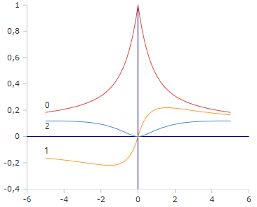
Bessel-Ie Functions (Order 0,1,2)
The exponentially scaled functions show controlled growth without numerical overflows even for large z values.
Characteristic Properties
- Ie₀(z) starts at 1, then decreases
- Ieₙ(z) with n > 0 starts at 0
- Asymptotically: ~ 1/√(2πz)
- No exponential overflows
Detailed Description of the Bessel-Ie Function
Mathematical Definition
The exponentially scaled modified Bessel function Ieᵥ(z) is a numerically stabilized version of the modified Bessel function Iᵥ(z). It was developed to solve the numerical problems of exponential growth.
Using the Calculator
Enter the order ν (integer) and the argument z (positive real number). The Ie version is particularly suitable for large z values.
Numerical Background
The development of exponentially scaled Bessel functions was a response to the challenges of scientific computing. While Iᵥ(z) grows exponentially for large z and causes overflows, Ieᵥ(z) remains within controlled limits.
Properties and Applications
Numerical Applications
- Scientific computing with large parameters
- Numerical libraries (MATLAB, SciPy, GSL)
- Simulation of physical systems
- Statistical calculations
Mathematical Properties
- Bounded growth for large z
- Asymptotically: ~ 1/√(2πz)
- Symmetry: Ie₋ₙ(z) = Ieₙ(z) for integer n
- Monotonicity properties similar to standard version
Implementation Aspects
- Libraries: Standard in modern math libraries
- Precision: Maintained accuracy for all z ranges
- Performance: Optimized algorithms available
- Portability: Platform-independent implementations
Interesting Facts
- The Ie functions are standard in IEEE floating-point implementations
- For small z: Ieᵥ(z) ≈ e^(-z) (z/2)^ν / Γ(ν+1)
- Algorithms often use continued fractions for higher efficiency
- Important in Monte Carlo simulations with large parameters
Calculation Examples and Comparisons
Small Argument
z = 1:
I₀(1) ≈ 1.266
Ie₀(1) ≈ 0.466
Medium Argument
z = 10:
I₀(10) ≈ 2815.7
Ie₀(10) ≈ 0.1278
Large Argument
z = 100:
I₀(100) → Overflow
Ie₀(100) ≈ 0.0398
Computational Comparison
Standard Iᵥ(z) Problems
Exponential Growth:
I₀(50) ≈ 1.1 × 10²¹
I₀(100) ≈ 1.1 × 10⁴²
I₀(700) → Overflow
Problem: Numerical overflows significantly limit the usable range.
Ieᵥ(z) Solution
Controlled Behavior:
Ie₀(50) ≈ 0.0564
Ie₀(100) ≈ 0.0398
Ie₀(700) ≈ 0.0151
Advantage: Stable computation for arbitrarily large arguments.
Algorithmic Implementation
Numerical Methods
- Continued Fractions: For large z and small ν
- Miller's Algorithm: For medium z ranges
- Series Expansion: For small z
- Uniform Asymptotic: For large ν
Software Implementations
- GSL: GNU Scientific Library
- Boost: C++ Boost Math Library
- SciPy: Python scientific computing
- MATLAB: Built-in besseli function with scaling
|
|
|
|