Calculate Bessel-Ke Function
Online calculator for the exponentially scaled modified Bessel function Keᵥ(z) of the second kind - Numerically stable solution for large arguments
Bessel-Ke Function Calculator
Exponentially Scaled K-Function
The Keᵥ(z) or exponentially scaled modified Bessel function provides numerical stability for extremely small values.
Bessel-Ke Function Curve
Mouse pointer on the graph shows the values.
The exponentially scaled form eliminates numerical problems for large z.
Why exponential scaling for the K-function?
The exponentially scaled modified Bessel-K function solves specific numerical challenges:
- Extreme decay: Prevents underflow for large z
- Exponential factor: Keᵥ(z) = e^z Kᵥ(z)
- Numerical robustness: Stable computation for all z ranges
- Scientific computing: Standard in numerical libraries
- Precision preservation: Avoids rounding errors
- Algorithm efficiency: Optimized implementations
|
|
Numerical advantages of exponential scaling
The exponentially scaled K-function offers crucial numerical improvements:
Problem with standard Kᵥ(z)
- Exponential decay ~ e^(-z)
- Underflow at z > ~700
- Loss of numerical precision
Solution through Keᵥ(z)
- Scaled value range without underflow
- Stable computation for arbitrarily large z
- Preserved relative accuracy
Formulas for the Bessel-Ke Function
Definition
Exponentially scaled modified Bessel function
Relationship to Kᵥ
Inversion of scaling
Integral Representation
Scaled integral form for Re(z) > 0
Asymptotic Form
For large z (without exponential decay)
Recurrence Formula
Same recurrence as unscaled version
Symmetry Property
Symmetry with respect to order
Behavior as z → 0
Scaled singularity at origin
Special Values
Important Values
Symmetry Properties
For all real ν
Singularity at z = 0
For all ν ≥ 0 (scaled)
Behavior as z → ∞
Algebraic decay (scaled)
Application Areas
Numerical stability, large parameters, scientific computing, precision algorithms.
Bessel-Ke vs. Bessel-K Comparison
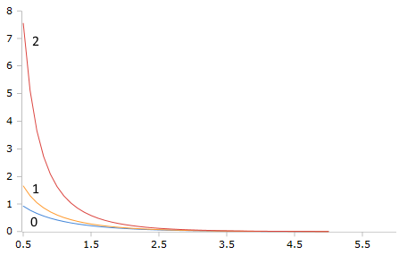
Bessel-Ke Functions (Order 0,1,2)
The exponentially scaled K-functions show algebraic decay behavior without numerical underflow even for very large z values.
Characteristic Properties
- Keᵥ(z) → ∞ for z → 0⁺ (scaled singularity)
- Keᵥ(z) ~ √(π/2z) for z → ∞
- Asymptotically: ~ 1/√z instead of e^(-z)
- Numerically stable for all z ranges
Detailed Description of the Bessel-Ke Function
Mathematical Definition
The exponentially scaled modified Bessel function Keᵥ(z) is a numerically stabilized version of the modified Bessel-K function. It was developed to solve the numerical problems of extreme exponential decay.
Using the Calculator
Enter the order ν (integer) and the argument z (positive real number). The Ke version is particularly suitable for large z values and numerical stability.
Numerical Background
The development of exponentially scaled K-functions was a response to the extreme numerical challenges in computing Kᵥ(z) for large z. While Kᵥ(z) decays exponentially to 0 and causes underflow, Keᵥ(z) remains numerically manageable.
Properties and Applications
Numerical Applications
- Scientific computing with extreme parameters
- High-precision numerics (IEEE floating-point)
- Simulation of physical systems at large distances
- Statistical calculations with wide parameter ranges
Mathematical Properties
- Algebraic decay behavior ~ 1/√z
- Singularity at z = 0 (scaled)
- Symmetry: Ke₋ᵥ(z) = Keᵥ(z)
- Monotonicity properties similar to standard K-version
Implementation Aspects
- Libraries: Standard in modern math libraries
- Precision: Maintained accuracy for large z
- Performance: Optimized algorithms available
- Robustness: Avoids numerical underflow
Interesting Facts
- The Ke-functions are essential in modern numerical libraries
- For large z: Keᵥ(z) ≈ √(π/2z) instead of Kᵥ(z) ≈ √(π/2z) e^(-z)
- Algorithms often use special recurrence formulas for efficiency
- Important in numerical simulations with extreme parameters
Calculation Examples and Scaling Comparisons
Small Argument
z = 1:
K₀(1) ≈ 0.421
Ke₀(1) ≈ 1.144
Medium Argument
z = 10:
K₀(10) ≈ 1.78×10⁻⁵
Ke₀(10) ≈ 0.399
Large Argument
z = 100:
K₀(100) → Underflow
Ke₀(100) ≈ 0.126
Computational Comparison: Standard vs. Scaled
Standard Kᵥ(z) Problems
Exponential decay:
K₀(50) ≈ 3.4 × 10⁻²³
K₀(100) ≈ 4.7 × 10⁻⁴⁵
K₀(700) → Underflow
Problem: Numerical underflow significantly limits the usable range.
Keᵥ(z) Solution
Controlled behavior:
Ke₀(50) ≈ 0.178
Ke₀(100) ≈ 0.126
Ke₀(700) ≈ 0.048
Advantage: Stable computation for arbitrarily large arguments.
Physical Interpretation and Applications
Heat Conduction (scaled)
Scaled temperature distribution:
T_scaled(r) = A Ke₀(r/λ)
Numerically stable for large distances
Advantage: Computation possible even at very large distances.
Electromagnetic Fields
Scaled field decay:
E_scaled(r) ∝ Ke₀(r/δ)
Precise computation at large distances
Application: Far-field calculations and shielding effects.
Numerical Computation and Algorithms
Computation Methods
- Series Expansion: For small z (scaled coefficients)
- Asymptotic Expansion: For large z (simplified by scaling)
- Recurrence Relations: Stable for all z ranges
- Continued Fractions: Optimized convergence
Software Implementations
- GNU GSL: Optimized Ke-functions
- Boost Math: C++ template library with scaling
- SciPy: Python scipy.special.kve
- MATLAB: Built-in besselk with scaling option
|
|
|
|