Calculate Bessel-Y Function
Online calculator for the Bessel function Yᵥ(z) of the second kind - Neumann function for oscillating cylindrical wave solutions
Bessel-Y Function Calculator
Bessel Function of the Second Kind
The Yᵥ(z) or Neumann function shows singular behavior at z = 0 and complements the J-function as a complete solution system.
Bessel-Y Function Curve
Mouse pointer on the graph shows the values.
The Y-function shows characteristic singularity at z = 0 and oscillates for large z.
|
|
Why is the Y-function singular at z = 0?
The Bessel function of the second kind complements the J-function to form a complete solution system:
- Linear independence: Yᵥ(z) is linearly independent of Jᵥ(z)
- Complete system: y = C₁Jᵥ(z) + C₂Yᵥ(z)
- Necessary singularity: Without singularity, the system would be incomplete
- Physical meaning: Describes outgoing waves
- Boundary conditions: Important for exterior problems
- Asymptotics: Yᵥ(z) ~ √(2/πz) sin(z - πν/2 - π/4)
Applications of the Neumann Function
The Bessel-Y function is essential for exterior boundary value problems and wave propagation:
Radiation Problems
- Antenna radiation into free space
- Electromagnetic wave propagation
- Acoustic radiation from sources
Exterior Regions
- Scattering from cylindrical objects
- Far-field approximations
- Infinite domain problems
Formulas for the Bessel-Y Function
Definition (Neumann)
Definition via Bessel functions of the first kind
For integer n
Limit definition for integer orders
Asymptotic Form
For large z (oscillating behavior)
Recurrence Formulas
Same recurrence relations as J-functions
Wronskian Determinant
Proves linear independence of Jᵥ and Yᵥ
Symmetry Property
For integer n
Behavior as z → 0
Singularity at origin for ν > 0
Special Values
Important Values
Symmetry Properties
For integer n
Singularity at z = 0
For all ν > 0
Behavior as z → ∞
Oscillating behavior
Application Areas
Radiation problems, scattering, exterior boundary conditions, wave propagation.
Bessel-Y Oscillation Pattern with Singularity
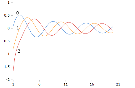
Bessel-Y Functions (Order 0,1,2)
The Y-functions show characteristic singularities at z = 0 and oscillating behavior for large z with phase shift relative to J-functions.
Characteristic Properties
- Yᵥ(z) → -∞ for z → 0⁺ (ν > 0)
- Y₀(z) ~ -(2/π) ln(z) for small z
- Asymptotically: ~ √(2/πz) sin(...)
- 90° phase shift relative to J-functions
Detailed Description of the Bessel-Y Function
Mathematical Definition
The Bessel function of the second kind Yᵥ(z), also known as the Neumann function, is the second linearly independent solution of the Bessel differential equation. It shows singular behavior at z = 0 and, together with Jᵥ(z), completes the fundamental solution system.
Using the Calculator
Enter the order ν (integer) and the argument z (positive real number). The graph stretch parameter controls the X-axis scaling for optimal oscillation display.
Historical Background
The Y-functions were systematically studied by Carl Neumann (1832-1925), which is why they are also called Neumann functions. They are essential for the complete description of physical systems with cylindrical symmetry.
Properties and Applications
Physical Applications
- Antenna radiation and electromagnetic wave propagation
- Acoustic radiation from cylindrical sources
- Scattering from cylindrical objects (exterior region)
- Far-field approximations in wave theory
Mathematical Properties
- Oscillating behavior with damping amplitude
- Singularity at z = 0 for all ν ≥ 0
- Linear independence from Jᵥ(z)
- 90° phase shift relative to J-functions
Numerical Aspects
- Stability: Numerically challenging near z = 0
- Algorithms: Special methods for small z values
- Accuracy: High precision for z > 0.1
- Efficiency: Recurrence formulas for adjacent orders
Interesting Facts
- Y₀(z) describes the logarithmic potential in 2D systems
- The zeros lie between those of the corresponding J-functions
- Y-functions are essential for Green's functions
- They describe outgoing waves in scattering theory
Calculation Examples and Singularity Behavior
Small Argument
z = 0.1:
Y₀(0.1) ≈ -1.534
Y₁(0.1) ≈ -6.459
Medium Argument
z = 2:
Y₀(2) ≈ 0.510
Y₁(2) ≈ -0.107
Large Argument
z = 20:
Y₀(20) ≈ -0.066
Asymptotic behavior
Detailed Physical Applications
Antenna Radiation
Cylindrical antennas:
H(r,φ,z) = [AJ_m(kr) + BY_m(kr)] e^(imφ) e^(ikz)
Y-term for outgoing waves
Example: Dipole antenna with cylindrical radiation pattern.
Scattering Problems
Cylinder scattering:
ψ_scattered ∝ Y_m(kr) e^(imφ)
For large distances from scatterer
Example: Electromagnetic scattering from conducting cylinders.
Mathematical Properties and Relations
Asymptotic Behavior
For large z:
Yᵥ(z) ~ √(2/πz) sin(z - πν/2 - π/4)
For small z (ν > 0):
Yᵥ(z) ~ -Γ(ν)/π (2/z)^ν
Special case: Y₀(z) ~ -(2/π) ln(z) for small z.
Relations to Other Functions
Wronskian determinant:
W[Jᵥ, Yᵥ] = 2/(πz)
Relation to Hankel functions:
H^(1)_ν(z) = Jᵥ(z) + iYᵥ(z)
Significance: Fundamental solution system with Jᵥ(z).
Special Orders and Limiting Cases
Order ν = 0
Y₀(z) - Fundamental solution:
Logarithmic singularity at z = 0
Application: 2D problems, logarithmic potentials.
Order ν = 1
Y₁(z) - First derivative:
Important for gradient problems
Application: Dipole radiation characteristics.
Numerical Computation and Algorithms
Computation Methods
- Series Expansion: For medium z (careful near z → 0)
- Asymptotic Expansion: For large z ≥ 25
- Recurrence Relations: For adjacent orders
- Miller's Algorithm: For stable backward recurrence
Software Implementations
- GNU GSL: High-precision Y-functions
- Boost Math: C++ template library
- SciPy: Python scipy.special.yn
- MATLAB: Built-in bessely function
|
|
|
|